Divise Clustering with HiPart 

Author:: Sotiris Tasoulis

Divisive Clustering and Visualization 

Herein is an example of the recent HiPart library for divisive clustering (Anagnostou et al. (2022)). In this tutorial, we will perform divisive clustering through one of the methods provided by the library, and we will examine it’s static visualizations options. There is an interactive plot tool provided by the package as well, but we will not cover it here. Initially we load the required libraries for this example, mainly the sklearn datasets and matplotlib for ploting.

# install HiPart using pip
# %pip install HiPart

import numpy as np
import pandas as pd
import matplotlib.pyplot as plt

from HiPart.clustering import dePDDP
from HiPart import visualizations as hvs

from sklearn.datasets import make_blobs
from sklearn.datasets import load_iris
from sklearn.datasets import load_linnerud

The iris example 

For consistency (and historical reasons :) ) we start with an example on clustering the iris dataset. The algorithm of choice here is dePDDP because it provides efficient density clustering and its parameterization unveils interesting aspects (S. K. Tasoulis, Tasoulis, and Plagianakos (2010)). The actual number of clusters is given (3), along with a “bandwidth” parameter that affects the sensitivity of the kernel density estimation, similarly to the bin_size parameter we usually provide to histograms. The basic attribute of this algorithm is that it clusters the data based on such one dimensional density estimations. Since, the clustering is divisive the algorithm generate binary splits thus, in contrast to other clustering methods, it is straight forward to define parameters such as the smallest size of cluster allowed, and how uneven should the resulting subclusters be. These are controlled by the “min_sample_split” and “percentile” parameters respectively.

data = load_iris()
Y = data.target
X = data.data

clustered_class = dePDDP(max_clusters_number=3, bandwidth_scale=0.5, percentile=0.2, min_sample_split=5)

clu_res = clustered_class.fit(X)

# clu_res.output_matrix
m = hvs.split_visualization(clu_res)

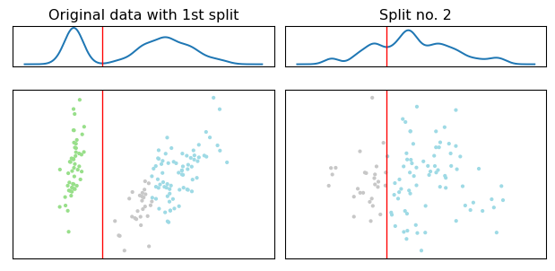
Divisive Clustering Example for 3 clusters

Notice:

The output_matrix output:

It can be very useful to get the whole tree structure in the form of a matrix. Each row represents a data point and each column cluster ids (predicted labels). More precisely each column contain the clustering ids to a corresponding iterative step of the clustering procedure, so the first column contains the clustering ids for a binary split, then the second the ids after the second break (cluster ids for three clusters) and the last column the final cluster ids according to the desired number of cluster given to the algorithm as input.

Lets change the desired number of clusters

The dePDDP algorithm is deterministic. In practice this means than when we rerun the algorithm “allowing” it to retrieve a higher number of clusters we just relax the stopping criterion. The algorithm will choose to split further a leaf node from the previous clustering result.

clustered_class = dePDDP(max_clusters_number=5, bandwidth_scale=0.5, percentile=0.2, min_sample_split=5)

clu_res = clustered_class.fit(X)
m = hvs.split_visualization(clu_res)

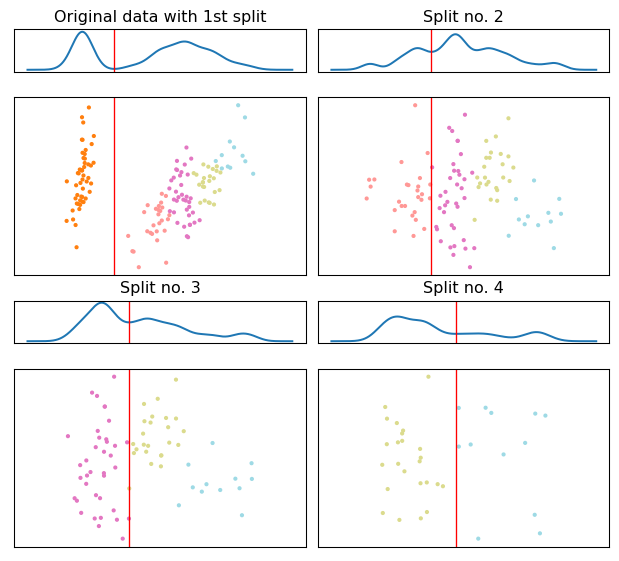
Divisive Clustering Example for 5 clusters

Simplicity, Sensitivity 

Setting up the parameters for dePDDP is super simple to understand but can be tricky as well. In practice, there are two dominant parameters that need to be specified carefully since they interact. For example the “number of clusters” parameter can be skipped completely. This will also allow us to use the algorithm for cluster number estimation. However, the bandwidth selection for the kernel density estimation could greatly affect the results in this case.

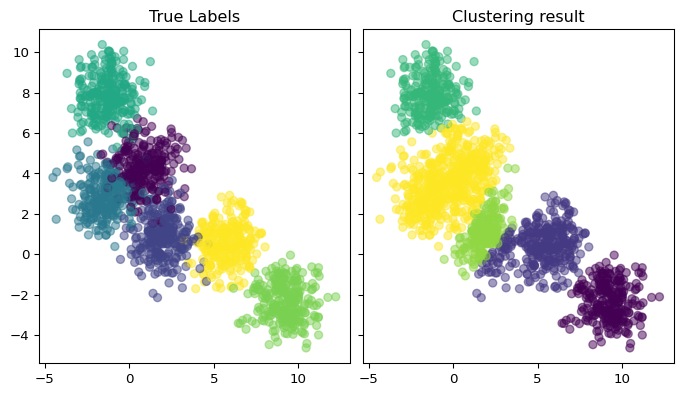
In the following example, we only set the “bandwidth_scale” parameter and the algorithm estimate the number of clusters itself. We plot the results along with the “true labels”. We observe that two clusters have great scale of overlap constituting in practice one cluster with double the size. The algorithm identifies it as one cluster and provides a reasonable estimate for the number of cluster in this example.

X, y = make_blobs(n_samples=1500, centers=6, random_state=0)

clustered_class = dePDDP(bandwidth_scale=1.5)

# get only the predicted class
clu_res = clustered_class.fit_predict(X)

fig, (ax1, ax2) = plt.subplots(1, 2, constrained_layout=True, sharey=True)
ax1.scatter(X[:,0], X[:,1], c=y, alpha=0.5)
ax1.set_title('True Labels')
ax2.scatter(X[:,0], X[:,1], c=clu_res, alpha=0.5)
ax2.set_title('Clustering result')

Text(0.5, 1.0, 'Clustering result')

Divisive Clustering Example

Dendrogram example 

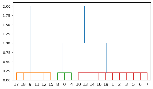
Yay, we can also plot dendrograms! Remember that divisive clustering operates in a top down fashion. The orange cluster has been split from the rest of the dataset first. Although there are no cluster similaries estimated here, we may assume that the green and red clusters are more similar to each other because they have been split later in the iterative procedure.

data = load_linnerud()
Y = data.target
X = data.data

clustered_class = dePDDP(max_clusters_number=3, bandwidth_scale=0.5, percentile=0.1, min_sample_split=1)

clu_res = clustered_class.fit(X)
m = hvs.dendrogram_visualization(clu_res)

Why bother?

Speed and efficiency comparison

In this example we will test HiPart for high dimensional data to expose the computational advantages of divisive over agglomerative clustering. We employ the super simple iPDDP algorithm (S. Tasoulis and Tasoulis (2008)) as we expect extensive data sparsity and a minimal deegre of cluster overlap, so the distance based clustering criterio seems more appropriate than the density one. We also use a dataset with uneven clusters to make the comparison more interesting.

from HiPart.clustering import iPDDP
from sklearn.cluster import AgglomerativeClustering
from sklearn.cluster import KMeans
import time
from sklearn import metrics


# generate the dataset
X, y = make_blobs(n_samples=[5000,2000,1000,500,500,200,100], centers=None, n_features= 1000,cluster_std=20,random_state=2)

# --------------
# set the model
clustered_class = iPDDP(max_clusters_number=7, percentile=0.1, min_sample_split=5)

st = time.time()
iPDDP_res = clustered_class.fit_predict(X)
et = time.time()
iPDDP_elapsed_time = et - st

# --------------
# set the model
Agglo_model = AgglomerativeClustering(n_clusters=7,linkage='average')

st = time.time()
Agglo_res = Agglo_model.fit_predict(X)
et = time.time()
Agglo_elapsed_time = et - st

# --------------
# set the model
kmeans_model = KMeans(n_clusters=7, random_state=0 )

st = time.time()
kmeans_res = kmeans_model.fit_predict(X)
et = time.time()
kmeans_elapsed_time = et - st

# Measure clustering efficiency as well with the Ajusted Rand Index metric
iPDDP_ARS = metrics.adjusted_rand_score(y, iPDDP_res)
agglo_ARS = metrics.adjusted_rand_score(y, Agglo_res)
kmeans_ARS = metrics.adjusted_rand_score(y, kmeans_res)

results = pd.DataFrame({"method" : ["iPDDP","Agglo","kmeans"], "Seconds" : [iPDDP_elapsed_time, Agglo_elapsed_time,kmeans_elapsed_time], "ARS" : [iPDDP_ARS,agglo_ARS,kmeans_ARS] })

print(results)

   method    Seconds       ARS
 iPDDP   2.134749  0.999651
 Agglo  30.910616  0.975736
kmeans   5.666819  0.583536

Anagnostou, Panagiotis, Sotiris Tasoulis, Vassilis Plagianakos, and Dimitris Tasoulis. 2022. “HiPart: Hierarchical Divisive Clustering Toolbox.” arXiv. https://doi.org/10.48550/ARXIV.2209.08680.

Tasoulis, S. K., D. K. Tasoulis, and V. P. Plagianakos. 2010. “Enhancing Principal Direction Divisive Clustering.” Pattern Recognition 43 (10): 3391–411. https://doi.org/https://doi.org/10.1016/j.patcog.2010.05.025.

Tasoulis, SK, and DK Tasoulis. 2008. “Improving Principal Direction Divisive Clustering.” In 14th ACM SIGKDD International Conference on Knowledge Discovery and Data Mining (KDD 2008), Workshop on Data Mining Using Matrices and Tensors.

Divise Clustering with HiPart

Divisive Clustering and Visualization

The iris example

Simplicity, Sensitivity

Dendrogram example